Your first analysis
This walks a single sample from file to exported numbers. It assumes you have installed the app and have either a trial or a license — viewing works without one, but gating does not.
1. Open a file
Section titled “1. Open a file”Click Open File in the toolbar (or press Ctrl+O), or drag an FCS file onto the window. You can open several at once.
The file appears in the file list on the left, and the app picks a starting pair of axes. Large files are fine — a million events opens in seconds.
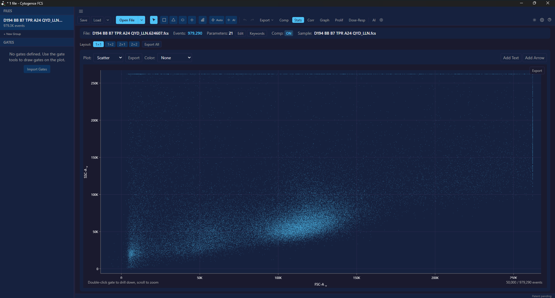
979,290 events, compensation applied, no gates yet. The footer reads
50,000 / 979,290 events — the plot draws a subsample for speed, while statistics
are computed over every event.
2. Check the axes and the scale
Section titled “2. Check the axes and the scale”Click either axis label to choose a parameter. Next to the parameter you choose a scale — and for fluorescence channels the right answer is almost never linear.
The app suggests a scale per channel. If a population is smeared against the axis or piled up at zero, the scale is wrong before the gate is wrong. See Scales and transforms.
3. Check the compensation
Section titled “3. Check the compensation”If the FCS file carries a spillover matrix from your acquisition software, the file is already compensated with it — the file list shows Comp beside it, and the file bar reads Comp: ON. If you have single-stain controls, the app can compute a matrix from them instead.
A file without a matrix opens uncompensated, which is fine for a scatter-only first look. See Compensation.
4. Draw your first gate
Section titled “4. Draw your first gate”Pick a gate tool from the gating toolbar — rectangle is the easiest to start with — and drag it around the population you want.
The gate appears in the gate list with its statistics. Draw the hygiene gates first, in the order a cytometrist expects: scatter to exclude debris, then singlets, then live cells.
5. Build a hierarchy
Section titled “5. Build a hierarchy”Double-click a gate to drill into it. The plot now shows only the events inside that gate, and any gate you draw is a child of it. Escape navigates back up.
This is what makes the statistics mean what you expect: a child population’s frequency is a percentage of its parent, and the breadcrumb above the plot shows you which parent you are in.
6. Let the AI propose the rest — optional
Section titled “6. Let the AI propose the rest — optional”Two different options, documented separately because they behave differently:
- AI-1 identifies a fixed list of immune populations on your machine, and declines the ones it cannot identify rather than guessing.
- The AI copilot takes a plain-language request (“gate CD4 T cell memory subsets”) and proposes a full strategy, step by step, for you to approve.
Neither applies anything without your click.
7. Read the statistics
Section titled “7. Read the statistics”The statistics table lists each population with its count and frequency, plus per-channel statistics. It updates as you move gates — adjust a boundary and the numbers follow.
See Statistics for what each column means and, importantly, what each percentage is a percentage of.
8. Export
Section titled “8. Export”- Statistics as CSV for your own analysis.
- Events as CSV, for all events or for one gate.
- Figures as SVG, PDF or PNG.
See Exporting.
9. Save the workspace
Section titled “9. Save the workspace”Ctrl+S saves the gate tree, each file’s compensation and your file names — not a copy of your data, a reference to it. Reopening restores the analysis. Saving works with or without a license.
If the FCS files have moved since you saved, the app lists them as missing and lets you locate each one, rather than failing. See Workspaces.
- The interface — what every panel is for
- Gating — all five gate types, editing, and automated gating
- Batch analysis — apply this strategy to a whole experiment