Gating

Gating requires a license. Viewing does not.

Gate types

Type	Use it for
Rectangle	Quick, axis-aligned regions. The fastest way to a first gate.
Polygon	Irregular populations — most real lymphocyte gates. Click to place vertices, close the shape to finish.
Ellipse	Roughly elliptical populations, where a polygon would be busywork.
Quadrant	Four regions from one crosshair. The classic two-marker readout.
Range	An interval on a single axis — useful on histograms and for time-based gates.

To abandon a gate part-way through drawing, press Escape, or click the Navigate tool (the cursor) at the left of the gating toolbar. (Before 0.2.2, only Navigate did.)

Gate and quadrant names

The app names a new gate Gate 1, Gate 2, and so on: the number is one more than the number of gates in the workspace. The gate tree is shared by every open file, so the numbering is not per file. Numbers are not reused or checked against existing names, so after deleting a gate you can end up with two gates of the same name — rename them if that matters to you.

A quadrant creates four gates, named by marker, x axis first:

Quadrant	Position	Example name
Q1	upper right	CD4+ CD8+
Q2	upper left	CD4- CD8+
Q3	lower left	CD4- CD8-
Q4	lower right	CD4+ CD8-

The marker is whatever the axis shows — the name you gave the channel, or else the marker from the file, or else the channel name — reduced to one clean marker word, so CD4 PE-Cy7 gives CD4. The signs are plain + and - (a hyphen), so scripts can match them. If either axis has no clean marker name — a detector such as FL2-A, a scatter channel, or a label like HLA-DR that already contains a hyphen — the quadrants are named by position instead: Q1: UR, Q2: UL, Q3: LL, Q4: LR.

Other names the app generates:

• A duplicated gate: the original name followed by (copy).
• A boolean gate: NOT Gate 1, or the operands joined by AND / OR, such as Gate 1 AND Gate 2.
• Auto clustering: Pop 1, Pop 2… for K-means and Gaussian mixtures, and Cluster 1, Cluster 2… for DBSCAN. Cluster… in the gate list names its populations Cluster 1, Cluster 2…
• Gates proposed by AI-1 or the copilot take the name in the proposal.

Generated names are the same in every interface language — English words, plain symbols. A gate’s name is data: it is saved in the workspace and written into statistics, gate templates and Gating-ML, so it should read the same for a script or for a colleague using the app in another language. A name you type, in any language, is kept exactly as written.

Renaming a gate

Double-click the gate’s name in the gate list, or click the pencil icon (Rename gate) on the selected row. Type the new name; Enter keeps it, Escape cancels, and clicking away also keeps it. An empty name is ignored. Renaming can be undone like any other gate change.

Editing a gate

Select it, then drag the whole gate or its vertices and handles. Statistics recompute as you move it, so you can watch a frequency settle rather than guessing where the boundary belongs.

• Delete or Backspace removes the selected gate. There is no confirmation — use undo if it was a mistake.
• Ctrl+Z undoes a gate change; Ctrl+Y (or Ctrl+Shift+Z) redoes it. On macOS, Cmd works as well as Ctrl.

Undo and redo cover changes to the gate tree — drawing, moving or resizing, deleting, renaming, recolouring, duplicating, moving a gate to another parent in the list, and importing a gate template. They do not cover compensation or plot settings. Opening a workspace starts a fresh undo history.

Hierarchy and drill-down

Double-click a gate to drill into it. The plot then shows only events inside that gate, and new gates become its children. Escape, or Go up (Esc) above the plot, goes back up. The breadcrumb above the plot always names where you are.

With more than one plot in the layout, Escape does not go up; use the Go up button instead.

This matters for interpretation, not just navigation: a child population’s frequency is a percentage of its parent. A tree that mixes denominators — some populations as a percentage of all events, some of their parent — is the single most common way a flow figure misleads. Drilling down is how you keep them consistent.

The conventional order is:

1. Scatter gate, to exclude debris
2. Singlets
3. Live cells, if you have a viability dye
4. Lineage gates below that

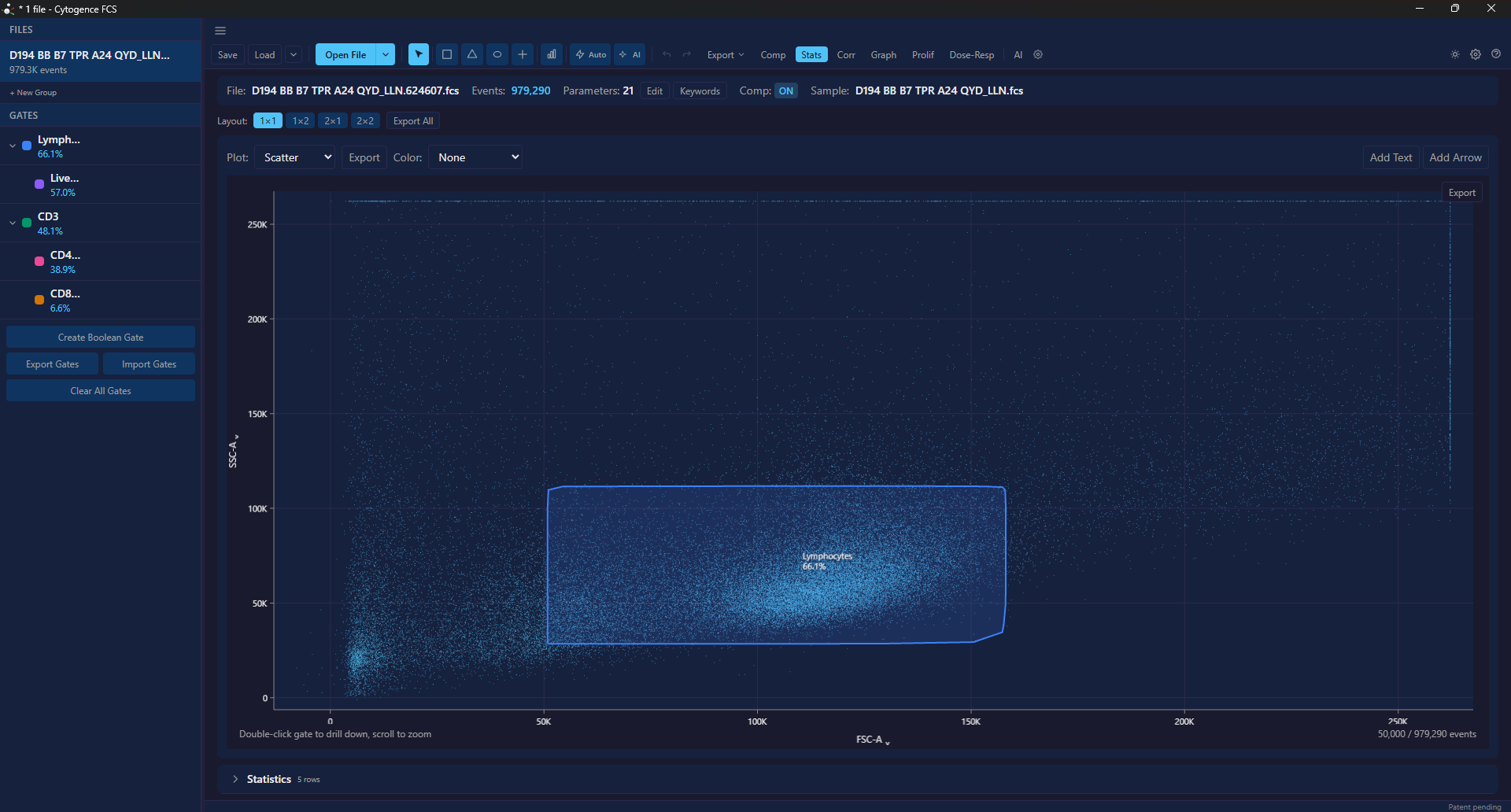
A hierarchy built by AI-1. Live lymphocytes nests under Lymphocytes; CD4 and CD8 nest under CD3.

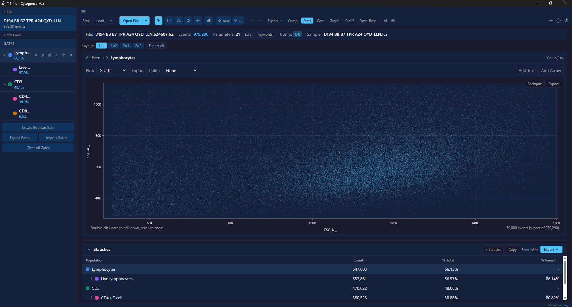
Drilled into Lymphocytes. The breadcrumb at the top reads All Events › Lymphocytes and Go up (Esc) — the plot now contains only events inside that gate, and anything drawn here becomes its child.

What the percentage beside each gate means

For a nested gate, the percentage in the gate list is of its parent and is labelled so — for example 86.1% of parent. For a top-level gate it is of all events in the file, shown as a bare percentage. With several files open, each file gets a compact entry, where a p after the number marks of parent.

The statistics table shows both denominators side by side; prefer it when the distinction matters.

Colours

Each gate gets a colour, used consistently in the gate list, in plots, and in exports — so a population in a figure is identifiable without a legend lookup.

Automated gating

Two independent routes, and they solve different problems.

Clustering

Auto in the gating toolbar clusters the events on the plot’s two axes and turns each cluster into an ellipse gate at the top level of the tree:

Algorithm	Character
K-means	Fast, wants a cluster count, assumes roughly round and similarly-sized clusters. Find Optimal k (Elbow Method) suggests a count.
DBSCAN	Finds clusters by density, handles odd shapes, does not need a count, and can label sparse events as noise — those are left out of the gates
GMM (Gaussian mixture)	Probabilistic and elliptical; better than K-means for overlapping populations. Find Optimal k (BIC) suggests a count.

Cluster… in the gate list is the other route: it groups cells by their whole marker profile at once, rather than by two channels, and makes each group a population. Import Labels does the same with per-cell labels from FlowSOM, Phenograph or your own script.

Clustering knows nothing about immunology — it finds structure. Whether a cluster is a population is your call, and the result is a set of gates you can then edit by hand like any other.

AI-1 and the copilot

Different from clustering: these propose named populations.

• AI-1 identifies a published list of immune populations on your machine and abstains on the rest.
• The AI copilot plans a whole strategy from a plain-language request, and you approve it step by step.

A note on compensation and gate coordinates

If you change compensation after drawing gates, check the gates. A gate is a region in a coordinate space, and changing the transform under it changes which events fall inside. Compensate first, then gate, whenever you can.